Creating Excel Reports Part 4 – Referencing Raw Data Using HLOOKUP

In the last tutorial, we were introduced to the VLOOKUP and were shown how powerful it can be when making reports in Excel. We created data tables and then reduced manual data entry by programming the report to use the tables to look up reoccurring values. As discussed previously, this makes it extremely easy to update certain types of information in your reports, such as phone numbers or hourly rates; once changed in the table the value can be automatically updated across all older data. In this tutorial we will be covering the other lookup command, HLOOKUP (Horizontal Look-up). HLOOKUP works very similar to VLOOKUP, but we will be using it in a completely different way. Rather then using it to check a table for a value and display associated information, we are going to use it to check the report for the current date, and then retrieve all of the information stored in “Misc” sheet for that date. This tutorial will be a little more advanced then the VLOOKUP one, I highly suggest you read through and review it first if you are new to lookup commands.

Step 1 – Set-up Your Data Table

We want the main report sheet to look-up data stored on the “misc” tab. Just like last time with VLOOKUP, we need to specify a data table for the function to search through. In this case it is the entire “Misc” sheet, so we first open the sheet, and then click the button where the row numbers and column letters intersect, see below:

Now everything is selected.  Just as before we click the name box just above the select-all button and enter a name for our data table, I chose “MiscData”:

Step 2 – The HLOOKUP Function

The anatomy of HLOOKUP is nearly identical to VLOOKUP, if you type =HLOOKUP( into any cell, the popup bubble will show you this:

If you remember the formula structure of VLOOKUP, they are almost identical, the only difference being that we now have “row_index_num” in place of “col_index_num”. As you may have guessed, HLOOKUP will search horizontally through the table, and once it finds the specified lookup_value it will display the data in the corresponding row from that column. Since we have selected the entire sheet for our data table in step 1, the row_index_num is identical to the row number on the sheet:

If you recall this is a typical column in Joe Transport’s “misc” sheet, note that when the column with the current day is found, it will display the information stored in the cell with the corresponding row index number. For example, let’s start with the “high” temperature field on the report:

So we want Excel to grab the date that is to be entered in cell B4 and look it up in the data table we defined earlier as MiscData then display the high temperature recorded in the “misc” sheet on the report page in cell N4. Now we define the variables in =HLOOKUP(lookup_value, table_array, row_index_num, [range_lookup]) as follows:

Lookup_value: B4 (the cell that contains the date)

Table_array: MiscData (as already defined)

Row_index_number: 3 (if you don’t see where this comes from look at the typical column image above)

[range_lookup]: FALSE (Just as the last tutorial, we will only be using false for our purposes)

When we put the formula in the cell it should look like this:

Now try it out, fill in a date on your report sheet and ensure the value is correctly selected. If you cannot get it to work for you, check Excel’s built-in Help Files.

Step 3 – Use HLOOKUP to Fill-out All Other Misc Data

Now that you have filed out one of the fields in the report, the same formula can be used to populate the other cells that reference raw data stored on the “misc” sheet, the only difference being the row_index_num specified. For filling out the large Work Activates box on the report, we would use the following formula:

=HLOOKUP(B4,MiscData,9,FALSE)

Similarly, for the number of cars under the Fleet Count section we would use

=HLOOKUP(B4,MiscData,17,FALSE)

The only fields that require a little extra trick to get working are the ones that require data to be referenced from the previous day, that is, Yesterdays workforce and vehicle fleet counts. For this to work, all we need to do is set the lookup_value equal to the current date minus one, or B4-1. Therefore, yesterday’s count of cars would be as follows:

=HLOOKUP(B4-1,MiscData,17,False)

We can go ahead and put the formula in all other cells that reference sheet “misc”. Note that it is important to not drag down formulas in this case, and to instead copy and paste them as text into adjacent cells. The reason for this is that Excel will not change the row_index_num when dragged, instead it will remain constant and all cells will display the same information. Here is a screenshot of my report page after I was done filling them in along with some arbitrary raw data, I also included some basic SUM() formulas:

This brings us to the end of this tutorial. We have now automated every piece of raw data stored in “misc” onto our main report page. We can change the displayed data from a previous date by simply changing the date on the report (in cell B4 for this example). In the next tutorial we will focus on entering shift data that will calculate and display revenue, expenses, and profits.

Creating Excel Reports Part 3 – Using Data Tables and VLOOKUP

Out of all the tutorials in this series this one is perhaps the most important, so be sure to pay close attention and put good effort into fully understanding VLOOKUP. This command (along with its sister command HLOOKUP-- to be covered in a later article) alone will make you a much more efficient Excel programmer. While I consider them essential for anything besides the most basic of reports, they are also useful for all kinds of data manipulation and even sometimes for quick analysis. These commands are used to search thorough and look up data in a given table or range. Once it finds the data specified, it will output any other value that is part of the same row adjacent to it. The easiest way to visualize this is by example:

Step 1 – Set-up your Data Tables

Similar to the first step of the previous tutorial, we need to create a new sheet. This sheet is going to be used for storing data tables containing employee contact numbers, rate of profit per hour for each vehicle (revenue), and rate of pay (expense) per hour. These tables need not be complicated, just one column for the independent variable and one or more for the dependant. Take a look at my tables below, the entries are just plain data, no formulas whatsoever.

Now that they are made, we need to create a label for each of them. To do this, simply highlight each table one at a time, then type in a unique label in the name field in the top left field and press enter.

Once you have all of your data tables named, click the drop down menu next to where you filled in the names to ensure that all of the names are there.

 Step 2 – Getting started with VLOOKUP

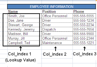
Do not be intimidated by the programming nature of VLOOKUP or HLOOKUP, they are simple once you break it down into small pieces; I’ll go into great detail the first time around. They are just formula that get entered into a cell, just like the SUM(a,b,c,….) or COUNT(a,b,c….) that you have likely used before. Here is the formula structure of VLOOKUP() taken right from Excel when you first enter it:

Lookup_value: Self explanatory, value (or cell) you want to search a data table for.

Table_array: The table that you want VLOOKUP to look though; enter the name that was used in step 1.

Col_index_num: Column index number, specifies which column of the table the data should be pulled from when VLOOKUP locates the lookup value.

[Range Lookup]: Don’t worry about this one; just make sure you always enter FALSE for its value.

Now that we know what each component means, let’s try a real example and begin programming the report. I want to make the position of an employee and their contact number to automatically fill themselves out in our Shift Data sheet after the employee’s name is entered. Lets start with the position first. I highlighted the position and contact columns blue in order to show that data is automatically entered in these cells rather then by the user.

Let’s put the formula into the first position cell:

As you can see, the correct formula is =VLOOKUP(B2, EMPLOYEES, 2, FALSE)

“B2” is the cell name that contains our lookup value, the employee’s name. “EMPLOYEES” is the name I gave my table back in step one, and “2” is the column index of the “position” data in the table.

Try entering an example of your lookup value, to make sure everything works properly. Next we are going to do the exact same thing for the contact number column, however the formula will be =VLOOKUP(B2, EMPLOYEES, 3, FALSE). Notice the only difference is “3”; the third column in our employee table contains the contact numbers. Now drag down both of these formulas all the way to the bottom of the sheet. Don’t worry about the #N/A that will appear, it just means that the lookup value (blank) wasn’t found.

The first part of the report is now fully automated. This reduces the amount of data that needs to be entered on a daily basis, increasing data entry efficiency and speed. Another major advantage of using data tables with VLOOKUP should now be noted, if a constant such as someone’s phone number changes, all that is needed to update the report is to change the number in the data table, the old numbers will all be updated automatically. If you still have problems using VLOOKUP please consult the Excel Help files, or search on the web for more resources.

Creating Excel Reports Part 2 – Getting Your Workbook Ready for Data Entry

In the previous part of this tutorial, I went through how to design the layout a professional summary report page, being careful to making it easy to read while packing lots of information into just a single page. At this point it is entirely possible to use this as a report template; you could enter all of the data into each field one at a time, calculate profits by hand, and then save a new excel file for each day. Unless your tracking a lemonade stand, you are going to need a much more efficient method of report generation. One of my cardinal rules for creating summary reports is that the main report page shall only require the current date to be entered into it; all of the rest of the report should generate itself. All information should be pulled from raw data stored in the other sheets of the same workbook.

Keeping your raw data separate from the main report offers two main advantages. Your raw data stays raw, that is it never gets directly modified. If a formula error or other mistake is made, your old data will always be there unchanged and is still safe for re-analysis. Secondly, this way of storing and referencing data allows you to regenerate a report from a past date instantly, all from the same report file. So if you ever need a copy of a report from a previous week, comments and all, you only need to change the date at the top of the page and then everything relevant to it will be displayed for printing.

Step 1 - Setting-Up New Sheets For Data

The first step is fairly easy. We need to create a new sheet for raw data. You can use as many different sheets as you see fit. I personally like to make one for each major type of data, and so in the case of our ongoing example of Joe Transport, I am going to use two. First I want a sheet that holds the comments and other miscellaneous information such as the weather and workforce, and then I want another sheet where raw shift data can be entered, one line for each employee’s completed work for that day. 

Starting with the miscellaneous data sheet, I choose to design it in a vertical sense. What I mean by this is that it will be a table that gets updated daily, with a new column holding the information for each day:

As you can see from above, the first column should be the labels for each entry field. Go ahead and set up a column for each day, I usually prepare a month or so at a time. Notice that the rows that hold text have been stretched out, this is to make it easier to display while you’re filling it in. You can set this up in any way you wish, with whatever information you deem important for your report.

Bonus Tip: To make the first (label) column stay put when scrolling with the rest of the (days) columns, click on the view tab, and select Freeze Panes à Freeze First Column. Now when you approach the later days of the month, you will still be able to see the label column on your screen when you scroll over.

Step 2 - Setting-Up Shift Report Data Entry

The next data tab we need to set up is the most important, as it will be used to calculate and track our financial information. It will compute the total revenue based on vehicle operating hours (using the generous simplification that a given vehicle generates a certain revenue per hour), as well as the total expenses based on total labor hours that must be paid out to employees on payday.

This data table is to work differently then the miscellaneous one. I find it easiest to track this type of information vertically, with a new row for each employee’s production for the day. Make sure you use the first column is reserved to enter the current date, but besides that it’s up to you to determine what information you need to collect. You can see my choices below, with a couple lines of example data included:

As you can see I really like to keep my daily raw data page layout as simple as possible. You may be wondering what all of the arrows next to my data labels are. These arrows are for a very useful feature called “Auto-Filter”. Once you have this sheet ready for data entry, highlight all of your column labels (row #1), then look up to your ribbon and go-to the Data tab,  then select Filter. You will now see the arrows. You can click these arrows anytime to sort the data below alphabetically, numerically, or select it to display only the rows that contain certain values in a chosen column. You can read more about this elsewhere if you really need too, but once you try experimenting with it you will very quickly figure out how it works; it’s quite simple.

This brings us to the end of this part of the tutorial. In the third part we will start to set up the report to organize and reference data from these entry sheets we have created using formulas as well as basic calculations.

Creating Excel Reports Part 1 – Designing a Professional Looking Report

When it comes to generating summary-type reports on a continual basis, such as a Total Production Summary, a weekly summary of revenue/expense activity, or similar, the best option is almost always Microsoft Excel. With a well organized and programmed Excel workbook, raw data can be entered directly into the sheet at regular intervals, and reports can be automatically generated by simply entering a date. Over the course of several tutorials, I will demonstrate how to design your report to look professional, be well organized, and to be fully automated to pull and display the data that you want it to.

For this and future tutorials I will be using an example of a fictitious transport company I have named “Joe’s Transport”. This is going to be a medium-sized company, which runs transport trucks, taxis, and busses in its business model. I will create a daily report that will allow Joe to track his day-to-day fleet usage, employee’s hours, total acquired revenue and total expenses broken down into each service offered by his company. This will allow him to monitor every part of his business, all in one compact, neat and professional report.   

Step 1 - Determine Exactly What You Need to Report

The very first step to designing an effective and efficient summary report in Excel is to figure out exactly what your report needs to display, before you even open up the program. I find it best to physically list out the required sections and subsections on paper. For my example of Joe’s Transport, I figure I will need to see the total number of employees working and total labor hours, the vehicle fleet being used, and a detailed breakdown of revenue gained from and total cost of operation for each service. I also require some additional information about each day that might effect the workday, such as weather conditions and room to record any additional comments or relevant incidents.

Step 2 - Design The Layout

Once we have established what we want our report to display, we need to decide how we want to display it. Having a good layout is absolutely critical. You information must be organized enough to read and interpret, while also being clean and professional looking. For a situation like our example, I would try to limit a Daily Summary to one or two pages, max.

It is now time to start the Excel work. First of all, I am assuming you know how to do some basic Excel tasks, such as merging cells, changing the font, and setting up boarders. If you run into any trouble with things like this just check out Excel’s help files or search the web. I find it easiest to first set-up the header, or top of your report. In the top part you are going to need at least the reports title and the current date underneath. Try and use lots of columns, that way you are sure to have room for adding as much information detail as you need later, then can always be merged if there are any extras. It is very important to make the label “Date:” a separate cell from the cell that you will actually enter the date in, as this will be later used for formulas. I chose to also include the weather conditions since this would be an important factor of business in Joe’s company. A small company logo in one of the top corners will help make the report look more professional. Here’s how I ended up formatting my header:

For my layout I plan on printing in “landscape” orientation rather then portrait, it’s up to you to decide how you would like to print your reports, but make this decision right away, or you will regret it later. Also please don’t laugh at my MS Paint logo; it’s only for the example!

 Next we must decide how we want each report element to be displayed. I like to first split the report area in half from top to bottom, and then split each half up into blocks.  Now I assign a section to each of the blocks. Try to visualize your report like this:

I can now choose roughly where I would like to place each of my sections. You can decide how to fill these up however you wish, I like to start from the top making small headers for the first two sections, then fill them out and move on to the next two, and so on. Make use of merging cells to make a layout that is clean and works for you, separate each section with some attractive boarders. I try to use a little color, something that matches the colors in to business logo. Try and keep the number of different colors to a minimum, too many makes the report look tacky and unprofessional.

I filled in my different sections and finally ended up with this:

Yours may look absolutely nothing like mine and that’s great, as long as it is well organized and looks professional. Don’t be afraid to experiment and play around a bit. In the next tutorial I will cover setting up a new sheet in the same work book to start entering data into that will be referenced into and be shown in the report sheet that we just created.

Three Quick Tips For Creating Excel Workbooks for Generating Reports

Microsoft Excel is an absolute powerhouse for data organization and analysis; it is an excellent option for both storing data and report generation. While building an Excel report spreadsheet is not overly complicated, there are certain quick tips you should know that will enhance your Excel reports and allow them to be much easier to use and read, as well as be more secure.

Tip #1: Use Separate Sheet for Data and the Excel Report

Excel reports are all about organization, so my number one tip is to keep all of your data on a different sheet (in the same workbook however) then the one that displays and calculates information (keep everything in the same workbook however) . Keeping all of your raw data away from calculations and formatting protects your raw data from being accidentally manipulated or changed, and keeps your report professional looking. Make cells in your Excel report sheet reference cells in your data, then use formulas to analyze it.

Tip #2: Protect Your Report Sheet and Use Data Validation

It is very easy to delete a formula in Excel by typing a value over it by accident. Do yourself a huge favor and save yourself much re-programming time by locking up your formula cells. After you have a formula entered into a cell, right click it and go to Format cells -> Protection. Now, once you have all of your cells protected go to the Review tab on the ribbon, and select "Protect Sheet" and lock it with an easy to remember password. Now that your sheet is locked, you can be safe from accidental clicks from yourself or anybody else. A similar feature you should take advantage of for your Excel reports is called Data Validation. Data Validation can be found under the Data tab in Excel 2007, it allows you to restrict the type of input a user can insert into it. For example you may want to only have a number between 1-100, or only names stored on a list under another sheet. For more specifics on Data Validation check out the Excel help files.

Tip #3: Learn How to Use the Function VLOOKUP( ), and Embrace it!

The VLOOKUP( ) function is absolutely essential for creating professional and efficient Excel reports. It is used to take the value of a given cell, look it up into a pre-made table, then set the value equal to the corresponding adjacent entry on the table. This may sound complicated, but really its not. For example, if we had a table that lists all employee names in one column, then next to it their phone numbers, we could use VLOOKUP( ) to automatically look-up and display the phone number each time you enter a employees name in the report!

As you can see in the above example, this very simple Excel report takes the name you enter (in blue), then automatically looks up the value of the phone number next to it in the table to the right, then displays it in the orange square. It may seem trivial in this example, but if you had a list of 100 people and needed to display their phone number every time you entered their name in your excel report, you will appreciate this feature. Check out Excel's help files to see how to use VLOOKUP () function, its not difficult!